Bayes' theorem
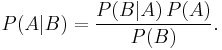
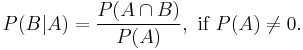
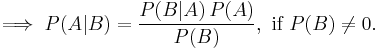
In probability theory and statistics, Bayes' theorem (alternatively Bayes' law or Bayes' rule) is a method of incorporating new knowledge to update the value of the probability of occurence of an event. To that end the theorem gives the relationship between the updated probability  , the conditional probability of
  given the new knowledge
  , and the probabilities of and ,
  and
and  , and the conditional probability of given ,
  . The theorem is named for Thomas Bayes (pronounced /ˈbeɪz/ or "bays").[1] In its most common form, Bayes' theorem is:
Contents |
Introductory example
If someone told you he had a nice conversation in the train, the probability it was a woman he spoke with is 50%. If he told you the person he spoke to was going to visit a quilt exhibition, it is far more likely than 50% it is a woman. Call  the event he spoke to a woman, and
  the event "a visitor of the quilt exhibition". Then:
 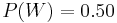 , but with the knowledge of the updated value is
  that may be calculated with Bayes' formula as:

in which  (man) is the complement of . As
 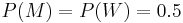 and
and 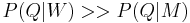 , the updated value will be quite close to 1.
Interpretation
Bayes' theorem has two distinct interpretations. In the frequentist interpretation it relates two representations of the probabilities assigned to a set of outcomes (conceptual inverses of each other). Both can be meaningful, so if only one is known Bayes' theorem enables conversion. In the Bayesian interpretation, Bayes' theorem is an expression of how degrees of belief should rationally be updated to account for evidence. The application of this view is called Bayesian inference, and is widely applied in fields including science, engineering, medicine and law.[2] The meaning of Bayes' theorem depends on the interpretation of probability ascribed to the terms:
Frequentist interpretation
In the frequentist interpretation, probability measures the proportion of trials in which an event (a subset of the possible outcomes) occurs. Consider events and . Suppose we consider only trials in which occurs. The proportion in which also occur is . Conversely, suppose we consider only trials in which occurs. The proportion in which also occur is . Bayes' theorem links these two quantities, with and the overall proportions of trials with and .
The situation may be more fully visualised with tree diagrams, shown to the right. For example, suppose that some members of a population have a risk factor for a medical condition, and some have the condition. The proportion with the condition depends whether those with or without the risk factor are examined. The proportion having the risk factor depends whether those with or without the condition are examined. Bayes' theorem links these two representations.
Bayesian interpretation
In the Bayesian (or epistemological) interpretation, probability measures a degree of belief. Bayes' theorem then links the degree of belief in a proposition before and after accounting for evidence. For example, suppose somebody proposes that a biased coin is twice as likely to land heads than tails. Degree of belief in this might initially be 50%. The coin is then flipped a number of times to collect evidence. Belief may rise to 70% if the evidence supports the proposition.
For proposition and evidence ,
-
- , the prior, is the initial degree of belief in .
- , the posterior, is the degree of belief having accounted for .
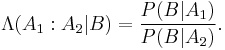
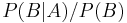 represents the support provides for .
For more on the application of Bayes' theorem under the Bayesian interpretation of probability, see Bayesian inference.
Forms
For events
Simple form
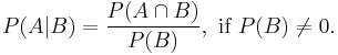
For events and , provided that  .
.
In a Bayesian inference step, the probability of evidence is constant for all models  . The posterior may then be expressed as proportional to the numerator:

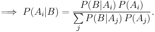
Extended form
Often, for some partition of the event space  , the event space is given or conceptualized in terms of
  and
and  . It is then useful to eliminate using the law of total probability:
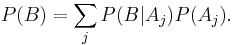
In the special case of a binary partition,
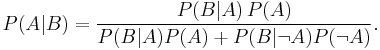
Three or more events
Extensions to Bayes' theorem may be found for three or more events. For example, for three events, two possible tree diagrams branch in the order BCA and ABC. By repeatedly applying the definition of conditional probability:

As previously, the law of total probability may be substituted for unknown marginal probabilities.
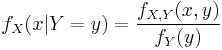
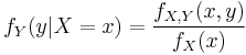
For random variables
Consider a sample space  generated by two random variables
  and
and  . In principle, Bayes' theorem applies to the events
  and
and  . However, terms become 0 at points where either variable has finite probability density. To remain useful, Bayes' theorem may be formulated in terms of the relevant densities (see Derivation).
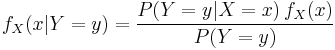
Simple form
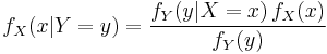
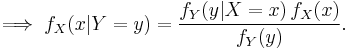
If is continuous and is discrete,
If is discrete and is continuous,
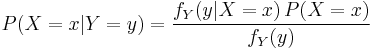
If both and are continuous,
Extended form
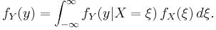
A continuous event space is often conceptualized in terms of the numerator terms. It is then useful to eliminate the denominator using the law of total probability. For  , this becomes an integral:
Bayes' rule
Under the Bayesian interpretation of probability, Bayes' rule may be thought of as Bayes' theorem in odds form.

Where
Derivation
For general events
Bayes' theorem may be derived from the definition of conditional probability:

For random variables
For two continuous random variables and , Bayes' theorem may be analogously derived from the definition of conditional density:
Examples
Frequentist example
An entomologist spots what might be a rare subspecies of beetle, due to the pattern on its back. In the rare subspecies, 98% have the pattern. In the common subspecies, 5% have the pattern. The rare subspecies accounts for only 0.1% of the population. How likely is the beetle to be rare?
From the extended form of Bayes' theorem,
![\begin{align}P(\text{Rare}|\text{Pattern}) &= \frac{P(\text{Pattern}|\text{Rare})P(\text{Rare})} {P(\text{Pattern}|\text{Rare})P(\text{Rare}) \, %2B \, P(\text{Pattern}|\text{Common})P(\text{Common})} \\[8pt]
&= \frac{0.98 \times 0.001} {0.98 \times 0.001 %2B 0.05 \times 0.999} \\[8pt]
&\approx 1.9\% \end{align}](/2012-wikipedia_en_all_nopic_01_2012/I/e09db424795cfda5ed764708b888430f.png)
Drug testing
Suppose a drug test is 99% sensitive and 99% specific. That is, the test will produce 99% true positive and 99% true negative results. Suppose that 0.5% of people are users of the drug. If an individual tests positive, what is the probability they are a user?
![\begin{align}
P(\text{User}|\text{%2B}) &= \frac{P(\text{%2B}|\text{User}) P(\text{User})}{P(\text{%2B}|\text{User}) P(\text{User}) %2B P(\text{%2B}|\text{Non-user}) P(\text{Non-user})} \\[8pt]
&= \frac{0.99 \times 0.005}{0.99 \times 0.005 %2B 0.01 \times 0.995} \\[8pt]
&\approx 33.2\%
\end{align}](/2012-wikipedia_en_all_nopic_01_2012/I/7266f2dcffd786af3ac5ce73963ffd18.png)
Despite the apparent accuracy of the test, if an individual tests positive, it is more likely that they do not use the drug than that they do.
This surprising result arises because the number of non-users is very large compared to the number of users, such that the number of false positives (0.995%) outweighs the number of true positives (0.495%). To use concrete numbers, if 1000 individuals are tested, there are expected to be 995 non-users and 5 users. From the 995 non-users,  false positives are expected. From the 5 users,
 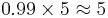 true positives are expected. Out of 15 positive results, only 5, about 33%, are genuine.
Historical remarks
Bayes' theorem was named after the Reverend Thomas Bayes (1702–61), who studied how to compute a distribution for the probability parameter of a binomial distribution (in modern terminology). His friend Richard Price edited and presented this work in 1763, after Bayes' death, as An Essay towards solving a Problem in the Doctrine of Chances.[3] The French mathematician Pierre-Simon Laplace reproduced and extended Bayes' results in 1774, apparently quite unaware of Bayes' work.[4] Stephen Stigler suggested in 1983 that Bayes' theorem was discovered by Nicholas Saunderson some time before Bayes.[5] Edwards (1986) disputed that interpretation.[6]
Bayes' preliminary results (Propositions 3, 4, and 5) imply the truth of the theorem that is named for him. Particularly, Proposition 5 gives a simple description of conditional probability:
- "If there be two subsequent events, the probability of the second b/N and the probability of both together P/N, and it being first discovered that the second event has also happened, from hence I guess that the first event has also happened, the probability I am right is P/b."
However, it does not appear that Bayes emphasized or focused on this finding. He presented his work as the solution to a problem:
- "Given the number of times in which an unknown event has happened and failed [... Find] the chance that the probability of its happening in a single trial lies somewhere between any two degrees of probability that can be named."[3]
Bayes gave an example of a man trying to guess the ratio of "blanks" and "prizes" at a lottery. So far the man has watched the lottery draw ten blanks and one prize. Given these data, Bayes showed in detail how to compute the probability that the ratio of blanks to prizes is between 9:1 and 11:1 (the probability is low - about 7.7%). He went on to describe that computation after the man has watched the lottery draw twenty blanks and two prizes, forty blanks and four prizes, and so on. Finally, having drawn 10,000 blanks and 1,000 prizes, the probability reaches about 97%.[3]
Bayes' main result (Proposition 9) is the following in modern terms:
- Assume a uniform prior distribution of the binomial parameter
 . After observing
  successes and
  failures,
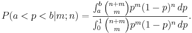
It is unclear whether Bayes was a "Bayesian" in the modern sense. That is, whether he was interested in Bayesian inference, or merely in probability. Proposition 9 seems "Bayesian" in its presentation as a probability about the parameter . However, Bayes stated his question in a manner that suggests a frequentist viewpoint: he supposed that a billiard ball is thrown at random onto a billiard table, and considered further billiard balls that fall above or below the first ball with probabilities and  . The algebra is of course identical no matter which view is taken.
Stephen Fienberg describes the evolution from "inverse probability" at the time of Bayes and Laplace, a term still used by Harold Jeffreys (1939), to "Bayesian" in the 1950s.[7] Ironically, Ronald A. Fisher introduced the "Bayesian" label in a derogatory sense.
Richard Price and the existence of God
Richard Price discovered Bayes' essay and its now-famous theorem in Bayes' papers after Bayes' death. He believed that Bayes' Theorem helped prove the existence of God ("the Deity") and wrote the following in his introduction to the essay:
- "The purpose I mean is, to shew what reason we have for believing that there are in the constitution of things fixt laws according to which things happen, and that, therefore, the frame of the world must be the effect of the wisdom and power of an intelligent cause; and thus to confirm the argument taken from final causes for the existence of the Deity. It will be easy to see that the converse problem solved in this essay is more directly applicable to this purpose; for it shews us, with distinctness and precision, in every case of any particular order or recurrency of events, what reason there is to think that such recurrency or order is derived from stable causes or regulations in nature, and not from any irregularities of chance." (Philosophical Transactions of the Royal Society of London, 1763)[3]
In modern terms this is an instance of the teleological argument.
See also
- Dempster–Shafer theory – generalization of Bayes' theorem
Notes
- ^ McGrayne, Sharon Bertsch. (2011). The Theory That Would Not Die, p. 10. at Google Books
- ^ Jaynes, Edwin T. (2003). Probability theory: the logic of science. Cambridge University Press. ISBN 9780521592710.
- ^ a b c d Bayes, Thomas, and Price, Richard (1763). "An Essay towards solving a Problem in the Doctrine of Chance. By the late Rev. Mr. Bayes, communicated by Mr. Price, in a letter to John Canton, M. A. and F. R. S.". Philosophical Transactions of the Royal Society of London 53 (0): 370–418. doi:10.1098/rstl.1763.0053. http://www.stat.ucla.edu/history/essay.pdf.
- ^ Daston, Lorraine (1988). Classical Probability in the Enlightenment. Princeton Univ Press. p. 268. ISBN 0-691-08497-1.
- ^ Stephen M. Stigler (1983), "Who Discovered Bayes' Theorem?" The American Statistician 37(4):290–296.
- ^ A. W. F. Edwards (1986), "Is the Reference in Hartley (1749) to Bayesian Inference?", The American Statistician 40(2):109–110
- ^ Fienberg, Stephen E. (2006).When Did Bayesian Inference Become “Bayesian”?.
References
- McGrayne, Sharon Bertsch. (2011). The Theory That Would Not Die: How Bayes' Rule Cracked The Enigma Code, Hunted Down Russian Submarines, & Emerged Triumphant from Two Centuries of Controversy. New Haven: Yale University Press. 13-ISBN 9780300169690/10-ISBN 0300169698; OCLC 670481486
Versions of the essay
- Bayes, Thomas; Price, Mr. (1763). "An Essay towards solving a Problem in the Doctrine of Chances.". Philosophical Transactions of the Royal Society of London 53 (0): 370–418. doi:10.1098/rstl.1763.0053.
- Barnard, G (1958). "Studies in the History of Probability and Statistics: IX. Thomas Bayes's An Essay Towards Solving a Problem in the Doctrine of Chances". Biometrika 45 (3–4): 296–315.. doi:10.1093/biomet/45.3-4.293.
- Thomas Bayes "An Essay towards solving a Problem in the Doctrine of Chances". (Bayes' essay in the original notation)
Commentaries
- G. A. Barnard (1958) "Studies in the History of Probability and Statistics: IX. Thomas Bayes' Essay Towards Solving a Problem in the Doctrine of Chances", Biometrika 45:293–295. (biographical remarks)
- Stephen M. Stigler (1982). "Thomas Bayes' Bayesian Inference," Journal of the Royal Statistical Society, Series A, 145:250–258. (Stigler argues for a revised interpretation of the essay; recommended)
- Isaac Todhunter (1865). A History of the Mathematical Theory of Probability from the time of Pascal to that of Laplace, Macmillan. Reprinted 1949, 1956 by Chelsea and 2001 by Thoemmes.
Additional material
- Bayesian Statistics summary from Scholarpedia.
- Laplace, Pierre-Simon. (1774/1986), "Memoir on the Probability of the Causes of Events", Statistical Science 1(3):364–378.
- Stephen M. Stigler (1986), "Laplace's 1774 memoir on inverse probability", Statistical Science 1(3):359–378.
- Jeff Miller, et al., Earliest Known Uses of Some of the Words of Mathematics (B). Contains origins of "Bayesian", "Bayes' Theorem", "Bayes Estimate/Risk/Solution", "Empirical Bayes", and "Bayes Factor".
- Weisstein, Eric W., "Bayes' Theorem" from MathWorld.
- Bayes' theorem at PlanetMath.
- A tutorial on probability and Bayes’ theorem devised for Oxford University psychology students
- A graphical explanation of the Bayes theorem.
- Bayes’ rule: A Tutorial Introduction by JV Stone.